主题切换
16.2 极值理论与尾部风险
名词解释:极值理论(Extreme Value Theory, EVT)
极值理论是统计学中专门研究随机变量极端值(极大值或极小值)分布的理论。在金融风险管理中,EVT 用于建模资产收益分布的尾部行为——这些极端事件虽然罕见,但对组合的影响是毁灭性的。标准正态分布假设会严重低估尾部风险,EVT 提供了一种更加科学的方法来估计极端损失的频率和规模。
一、极值理论核心分布:GEV 和 GPD
1.1 广义极值分布(GEV)
块极大值法(Block Maxima):将数据分成等大小的块,取每块的最大值(或最小值),用 GEV 分布拟合。
其中
:Fréchet 分布(厚尾),适用于金融收益率 :Gumbel 分布(指数尾) :Weibull 分布(薄尾/有界分布)
1.2 广义帕累托分布(GPD)
阈值超越法(Peaks-Over-Threshold, POT):对超过某个高阈值
其中
此处有展示代码展开 ▼
python
import numpy as np
import pandas as pd
from scipy import stats, optimize
import matplotlib.pyplot as plt

def fit_gpd(exceedances: np.ndarray) -> dict:
    """
    用极大似然估计拟合广义帕累托分布(GPD)。

    参数:
        exceedances: 超过阈值的超出量(正值)
    返回:
        包含 xi, beta, log_likelihood 的字典
    """
    def gpd_neg_loglik(params, data):
        xi, log_beta = params
        beta = np.exp(log_beta)  # 确保正值

        n = len(data)
        if abs(xi) < 1e-8:
            # xi ≈ 0 时的极限情况(指数分布)
            ll = -n * np.log(beta) - np.sum(data) / beta
        else:
            # 标准GPD对数似然
            if np.any(1 + xi * data / beta <= 0):
                return 1e10  # 惩罚不满足支撑域的参数
            ll = -n * np.log(beta) - (1 + 1/xi) * \
                 np.sum(np.log(1 + xi * data / beta))

        return -ll

    # 初始猜测:使用矩估计
    m = np.mean(exceedances)
    v = np.var(exceedances)
    xi0 = 0.5 * (1 - m**2 / v)
    beta0 = 0.5 * m * (1 + m**2 / v)

    result = optimize.minimize(
        gpd_neg_loglik,
        [xi0, np.log(beta0)],
        args=(exceedances,),
        method='Nelder-Mead',
        options={'maxiter': 2000}
    )

    xi_hat = result.x[0]
    beta_hat = np.exp(result.x[1])

    return {
        'xi': xi_hat,
        'beta': beta_hat,
        'log_likelihood': -result.fun,
        'convergence': result.success
    }

# ===== 合成数据最小示例(数据为模拟,机制真实)=====
np.random.seed(167)
_losses = np.abs(np.random.standard_t(3, 3000)) * 0.02
_exc = _losses[_losses > 0.03] - 0.03
_g = fit_gpd(_exc)
for _k, _v in _g.items():
print(f'{_k}: {_v}')点击展开可浏览运行结果
xi: 0.2356660528445306
beta: 0.020323954586812604
log_likelihood: 1832.9547941714693
convergence: True
1.3 阈值选择方法
此处有展示代码展开 ▼
python
import numpy as np

def threshold_selection(returns: np.ndarray,
                         method: str = 'mean_excess') -> float:
    """
    选择POT方法的阈值 u。

    方法 'mean_excess': 平均超出函数 (Mean Excess Function)
       e(u) = E[X - u | X > u],在线性区域选择阈值

    方法 'quantile': 取指定的分位数

    参数:
        returns: 收益率(以损失为正,即对多头用 -returns)
        method: 阈值选择方法
    返回:
        建议的阈值 u
    """
    if method == 'quantile':
        # 取90%或95%分位数
        return np.percentile(returns, 90)

    elif method == 'mean_excess':
        sorted_losses = np.sort(returns)
        n = len(sorted_losses)

        # 计算各候选阈值的平均超出量
        thresholds = np.linspace(np.percentile(returns, 80),
                                 np.percentile(returns, 98),
                                 50)
        mean_excess = []

        for u in thresholds:
            exceedances = sorted_losses[sorted_losses > u] - u
            if len(exceedances) > 10:
                mean_excess.append(np.mean(exceedances))
            else:
                mean_excess.append(np.nan)

        # 寻找线性区域的起始点
        # 简化:取使平均超出量开始线性增长的阈值
        diffs = np.diff(mean_excess)
        for i in range(len(diffs) - 1):
            if abs(diffs[i+1] - diffs[i]) < 0.01 * np.std(returns):
                return thresholds[i]

        return np.percentile(returns, 90)  # 默认

# ===== 合成数据最小示例(数据为模拟,机制真实)=====
np.random.seed(173)
_losses = np.abs(np.random.standard_t(3, 2000)) * 0.02
print('mean_excess 阈值:', round(threshold_selection(_losses, method='mean_excess'), 4))点击展开可浏览运行结果
mean_excess 阈值: 0.0367
二、Hill 估计量与尾部指数
2.1 Hill 估计量
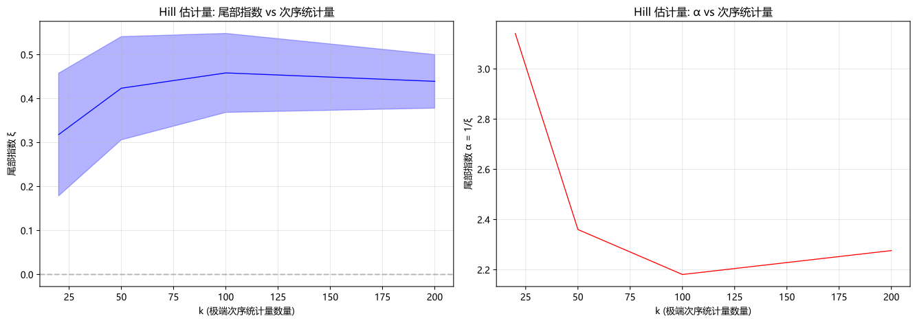
Hill 估计量是估计厚尾分布尾部指数最经典的方法。对于 Pareto 型尾部:
其中
2.2 实现与 Hill 图
此处有展示代码展开 ▼
python
import numpy as np
import pandas as pd

def hill_estimator(sorted_losses: np.ndarray,
                    k_values: list = None) -> pd.DataFrame:
    """
    Hill 估计量用于估计尾部指数。

    参数:
        sorted_losses: 降序排列的损失数据
        k_values: 用于估计的极端次序统计量数量列表
    返回:
        各 k 下的尾部指数估计 DataFrame
    """
    n = len(sorted_losses)
    if k_values is None:
        k_values = range(10, min(500, n // 10))

    results = []
    for k in k_values:
        if k >= n or k < 2:
            continue

        # Hill 估计量
        X_k_plus_1 = sorted_losses[k]  # 第 k+1 个次序统计量
        sum_log_ratio = np.sum(np.log(sorted_losses[:k] / X_k_plus_1))
        alpha_hat = k / sum_log_ratio
        xi_hat = 1.0 / alpha_hat

        # 近似标准误
        se_xi = xi_hat / np.sqrt(k)

        results.append({
            'k': k,
            'alpha': alpha_hat,
            'xi': xi_hat,
            'se_xi': se_xi,
            'xi_lower': xi_hat - 1.96 * se_xi,
            'xi_upper': xi_hat + 1.96 * se_xi
        })

    df = pd.DataFrame(results)

    # 绘制 Hill 图
    fig, axes = plt.subplots(1, 2, figsize=(14, 5))

    axes[0].plot(df['k'], df['xi'], 'b-', linewidth=1)
    axes[0].fill_between(df['k'], df['xi_lower'], df['xi_upper'],
                          alpha=0.3, color='blue')
    axes[0].axhline(y=0, color='gray', linestyle='--', alpha=0.5)
    axes[0].set_xlabel('k (极端次序统计量数量)')
    axes[0].set_ylabel('尾部指数 ξ')
    axes[0].set_title('Hill 估计量: 尾部指数 vs 次序统计量')
    axes[0].grid(True, alpha=0.3)

    axes[1].plot(df['k'], df['alpha'], 'r-', linewidth=1)
    axes[1].set_xlabel('k (极端次序统计量数量)')
    axes[1].set_ylabel('尾部指数 α = 1/ξ')
    axes[1].set_title('Hill 估计量: α vs 次序统计量')
    axes[1].grid(True, alpha=0.3)

    plt.tight_layout()
    plt.show()

    return df

# ===== 合成数据最小示例(数据为模拟,机制真实)=====
np.random.seed(179)
_losses = np.sort(np.abs(np.random.standard_t(3, 2000)) * 0.02)[::-1]
_h = hill_estimator(_losses, k_values=[20, 50, 100, 200])
print(_h.round(4).to_string() if hasattr(_h, 'to_string') else _h)点击展开可浏览运行结果
k   alpha      xi   se_xi  xi_lower  xi_upper
0   20  3.1414  0.3183  0.0712    0.1788    0.4578
1   50  2.3601  0.4237  0.0599    0.3063    0.5411
2  100  2.1811  0.4585  0.0458    0.3686    0.5483
3  200  2.2765  0.4393  0.0311    0.3784    0.5002
三、回测 VaR 的统计检验
3.1 Kupiec POF 检验
Kupiec (1995) 的比例失败检验(Proportion of Failures test)验证 VaR 例外发生的比例是否与置信水平一致。
零假设:实际的例外比例等于预期比例
3.2 Christoffersen 条件覆盖检验
此处有展示代码展开 ▼
python
from scipy import stats

import numpy as np

def var_backtest_validation(var_forecasts: np.ndarray,
                             actual_returns: np.ndarray,
                             confidence_level: float = 0.99) -> dict:
    """
    全面的 VaR 回测验证。

    包括:Kupiec POF 检验、Christoffersen 独立性检验、
          Christoffersen 条件覆盖检验。

    参数:
        var_forecasts: VaR 预测值序列(应为正值表示损失)
        actual_returns: 实际收益率(以损失为正,即 -returns)
        confidence_level: VaR 置信水平
    返回:
        检验统计量和 p 值
    """
    T = len(actual_returns)

    # 例外指示灯 I_t = 1 if Loss > VaR else 0
    exceptions = (actual_returns > var_forecasts).astype(int)
    N = exceptions.sum()
    alpha = 1 - confidence_level

    # 1. Kupiec POF 检验
    p_hat = N / T
    if p_hat == 0:
        lr_pof = -2 * (T * np.log(1 - alpha))
    elif p_hat == 1:
        lr_pof = -2 * (T * np.log(alpha))
    else:
        lr_pof = -2 * (np.log((1 - alpha)**(T - N) * alpha**N) -
                       np.log((1 - p_hat)**(T - N) * p_hat**N))

    p_value_pof = 1 - stats.chi2.cdf(lr_pof, 1)

    # 2. Christoffersen 独立性检验
    n00 = np.sum((exceptions[:-1] == 0) & (exceptions[1:] == 0))
    n01 = np.sum((exceptions[:-1] == 0) & (exceptions[1:] == 1))
    n10 = np.sum((exceptions[:-1] == 1) & (exceptions[1:] == 0))
    n11 = np.sum((exceptions[:-1] == 1) & (exceptions[1:] == 1))

    # 转移概率
    p01 = n01 / (n00 + n01) if (n00 + n01) > 0 else 0
    p11 = n11 / (n10 + n11) if (n10 + n11) > 0 else 0
    p = (n01 + n11) / (n00 + n01 + n10 + n11)

    if p01 == 0 or p11 == 0 or p == 0:
        lr_ind = 0
    else:
        lr_ind = -2 * (np.log((1 - p)**(n00 + n10) * p**(n01 + n11)) -
                       np.log((1 - p01)**n00 * p01**n01 *
                              (1 - p11)**n10 * p11**n11))

    p_value_ind = 1 - stats.chi2.cdf(lr_ind, 1)

    # 3. 条件覆盖检验 (Conditional Coverage)
    lr_cc = lr_pof + lr_ind
    p_value_cc = 1 - stats.chi2.cdf(lr_cc, 2)

    return {
        'T': T, 'N_exceptions': N, 'exception_rate': N / T,
        'expected_rate': alpha,
        'Kupiec_POF_LR': lr_pof, 'Kupiec_POF_pvalue': p_value_pof,
        'Christoffersen_Ind_LR': lr_ind,
        'Christoffersen_Ind_pvalue': p_value_ind,
        'Christoffersen_CC_LR': lr_cc,
        'Christoffersen_CC_pvalue': p_value_cc,
        'model_valid': p_value_cc > 0.05  # 5%显著性水平
    }

# ===== 合成数据最小示例(数据为模拟,机制真实)=====
np.random.seed(181)
_var = np.full(500, 0.025)
_act = np.abs(np.random.standard_t(4, 500)) * 0.015
_bt = var_backtest_validation(_var, _act)
for _k, _v in _bt.items():
print(f'{_k}: {_v if np.isscalar(_v) else str(_v)[:80]}')点击展开可浏览运行结果
T: 500
N_exceptions: 86
exception_rate: 0.172
expected_rate: 0.010000000000000009
Kupiec_POF_LR: 341.36761293742273
Kupiec_POF_pvalue: 0.0
Christoffersen_Ind_LR: 0.9551169209840396
Christoffersen_Ind_pvalue: 0.3284202401127434
Christoffersen_CC_LR: 342.3227298584068
Christoffersen_CC_pvalue: 0.0
model_valid: False
四、EVT 在压力测试中的应用
4.1 EVT-VaR 和 EVT-ES 的估计
基于 GPD 的 VaR 和 ES 估计(POT 方法):
此处有展示代码展开 ▼
python
from scipy import stats

import numpy as np

def evt_var_es(gpd_params: dict,
               threshold: float,
               n_total: int,
               n_exceedances: int,
               confidence_level: float = 0.99) -> dict:
    """
    基于 EVT (GPD-POT) 的 VaR 和预期亏损估计。

    参数:
        gpd_params: GPD 拟合结果 {'xi': ..., 'beta': ...}
        threshold: POT 阈值 u
        n_total: 总样本量
        n_exceedances: 超过阈值的样本量
        confidence_level: VaR 置信水平
    返回:
        EVT-VaR 和 EVT-ES
    """
    xi = gpd_params['xi']
    beta = gpd_params['beta']
    p = 1 - confidence_level

    # 尾部分布的非参数估计
    zeta_u = n_exceedances / n_total  # 超过阈值比例

    # EVT-VaR: u + β/ξ * [(n/ Nu * p)^{-ξ} - 1]
    if abs(xi) < 1e-8:
        var_evt = threshold - beta * np.log(p / zeta_u)
    else:
        var_evt = threshold + beta / xi * \
            ((p / zeta_u) ** (-xi) - 1)

    # EVT-ES: 预期亏损 = VaR / (1 - ξ) + (β - ξ*u) / (1 - ξ)  (ξ < 1)
    if xi < 1:
        if abs(xi) < 1e-8:
            es_evt = var_evt + beta
        else:
            es_evt = var_evt / (1 - xi) + (beta - xi * threshold) / (1 - xi)
    else:
        es_evt = np.inf  # ξ >= 1 时, ES 无穷大,分布过于厚尾

    return {
        'EVT_VaR': var_evt,
        'EVT_ES': es_evt,
        'gaussian_VaR': threshold + stats.norm.ppf(confidence_level) *
                         np.std(np.random.randn(n_total)),
        'tail_index_xi': xi
    }

# ===== 合成数据最小示例(数据为模拟,机制真实)=====
_e = evt_var_es(gpd_params={'xi': 0.2, 'beta': 0.008}, threshold=0.03,
                n_total=3000, n_exceedances=90)
for _k, _v in _e.items():
print(f'{_k}: {_v}')点击展开可浏览运行结果
EVT_VaR: 0.03982923758462069
EVT_ES: 0.05228654698077586
gaussian_VaR: 2.3552842973015107
tail_index_xi: 0.2
4.2 跨资产极值相依性
在实际压力测试中,仅考虑单一资产的极值风险是不够的——极端事件往往同时冲击多个资产。可以通过极值相依性(Extremal Dependence)指标来衡量:
- 尾部依赖系数(Tail Dependence Coefficient):
EVT 不仅为 VaR/ES 估计提供了更科学的尾部建模方法,也是压力测试设计的理论基石。掌握了 EVT 之后,我们就可以更有信心地构建极端但合理(Severe but Plausible)的压力情景。
常见误区
误区1:用正态分布外推极端行情。 金融收益厚尾是常态,正态假设会系统性低估 99% 分位以外的损失。
误区2:Hill 估计对阈值不敏感。 阈值过低引入非尾部样本(偏差),过高样本不足(方差大),必须做阈值稳定性分析。
误区3:VaR 回测只用连续性检验。 忽略违约聚类会漏检"风险模型在动荡期集体失效"这一最危险的形态,需叠加 Christoffersen 独立性检验。
误区4:EVT 万能。 EVT 依赖足够多的超阈值样本,对样本量小的新资产或制度突变场景同样脆弱。
本章要点
- EVT 两条路线:GEV(分块极大值)与 GPD(超阈值 POT)
- Hill 估计量用于尾部指数,阈值选择是偏差-方差权衡
- VaR 回测:Kupiec 覆盖率检验 + Christoffersen 独立性检验缺一不可
- 压力测试中用 EVT 尾部参数生成极端但合理的情景
跨模块延伸:VaR 体系