主题切换
3.5 可视化与探索
概念详解
可视化在量化中的多重角色
可视化远不只是"画好看的图"。在量化研究中,可视化是发现规律、诊断问题和沟通结果的三合一工具。
- 探索性分析:在建模前用图表发现数据中的模式和异常。散点图矩阵、分布图、时序图是发现非线性关系、异常值和结构性突变的最快手段。
- 诊断性分析:验证模型的假设和表现。残差图、Q-Q图、参数敏感性热力图帮助判断模型是否过拟合、违反哪些假设。
- 解释性沟通:将复杂的量化结果转化为可以理解的视觉故事。策略净值曲线、因子归因瀑布图、风险预算饼图让非技术背景的投资者也能理解策略逻辑。
名词解释:K线图
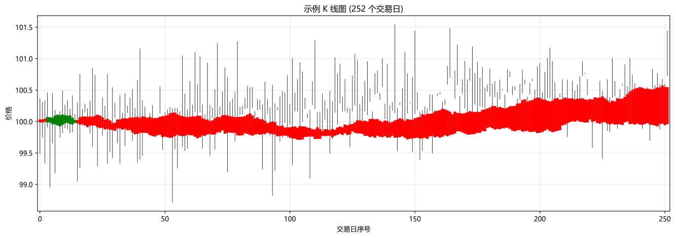
展示特定周期内开盘价、收盘价、最高价、最低价的图表,红色(或空心)表示上涨,绿色(或实心)表示下跌。
名词解释:热力图 (Heatmap)
用颜色深浅表示数值大小的矩阵图表。在量化中常用于展示相关性矩阵、因子IC矩阵、参数敏感性等。
名词解释:配对图 (Pair Plot)
展示多维数据中每对变量之间关系的矩阵图,对角线常放分布直方图或核密度估计。适合快速发现变量间的线性/非线性关系。
量化可视化的常用图表类型
| 图表类型 | 适用场景 | 常用库 |
|---|---|---|
| K线图 | 价格走势与形态分析 | matplotlib/mplfinance |
| 净值曲线 | 策略表现展示 | matplotlib |
| 相关性热力图 | 因子/资产间关系 | seaborn |
| 分布直方图 | 收益率分布诊断 | matplotlib/seaborn |
| 散点图 | 双变量关系探索 | matplotlib/seaborn |
| 箱线图 | 分组统计比较 | seaborn |
| 参数热力图 | 参数敏感性分析 | seaborn |
| 滚动折线图 | 时变特征展示 | matplotlib |
| 瀑布图 | 收益归因分解 | matplotlib |
| 树状图 | 资产层次聚类 | scipy/matplotlib |
金融图表的基本原则
- 颜色有含义:红色=下跌/亏损(中国红反之),绿色=上涨/盈利。不要随意反转颜色约定
- 标注关键事件:在时间序列图上标注市场重大事件(如2015年股灾、2020年3月崩盘)
- 对数坐标:对于跨越多个数量级的价格序列,对数坐标更合理
- 诚实轴:不要通过截断Y轴来夸大差异,不要用3D效果扭曲数据
- 网格线帮助阅读:适度的网格线(alpha=0.3)提升可读性
Python实战
案例1:绘制K线
此处有展示代码展开 ▼
python
import matplotlib.pyplot as plt
# 一键运行:用 demo 数据 df['Close'/'Open'/'High'/'Low'/'Volume'] 画 K 线图
fig, ax = plt.subplots(figsize=(14, 5))
prices = df[['Open', 'High', 'Low', 'Close']].reset_index(drop=True)
for i, row in prices.iterrows():
    color = 'red' if row['Close'] >= row['Open'] else 'green'
    ax.plot([i, i], [row['Low'], row['High']], 'black', linewidth=0.6)
    ax.plot([i, i], [row['Open'], row['Close']], color, linewidth=4)
ax.set_xlim(-1, len(prices))
ax.set_xlabel('交易日序号')
ax.set_ylabel('价格')
ax.set_title(f'示例 K 线图 ({len(prices)} 个交易日)')
ax.grid(True, alpha=0.3)
plt.tight_layout()
plt.show()
print(f"✅ K 线图已绘制 ({len(prices)} 根日K, 红涨绿跌)")点击展开可浏览运行结果
✅ K 线图已绘制 (252 根日K, 红涨绿跌)
案例2:专业量化可视化仪表盘
此处有展示代码展开 ▼
python
import matplotlib.pyplot as plt
import matplotlib.dates as mdates
import numpy as np
import pandas as pd
# 注:本案例纯 matplotlib, 不依赖 seaborn(浏览器沙箱不支持)。
from scipy import stats
from matplotlib.gridspec import GridSpec
import matplotlib.ticker as ticker

def quant_dashboard(price_data, strategy_nav=None, benchmark_nav=None,
                    returns=None, drawdowns=None, monthly_returns=None):
    """
    创建专业的量化策略仪表盘,整合多个关键诊断图表
    """
    # 设置中文字体
    plt.rcParams['font.sans-serif'] = ['SimHei', 'DejaVu Sans']
    plt.rcParams['axes.unicode_minus'] = False

    fig = plt.figure(figsize=(20, 14))
    gs = GridSpec(3, 3, figure=fig, hspace=0.35, wspace=0.35)

    # === 1. 价格走势与交易信号 (占据2列) ===
    ax1 = fig.add_subplot(gs[0, :2])
    ax1.plot(price_data.index, price_data['Close'], linewidth=0.8, color='#2c3e50', label='收盘价')

    # 如果提供了净值曲线
    if strategy_nav is not None:
        ax1_twin = ax1.twinx()
        ax1_twin.plot(strategy_nav.index, strategy_nav.values,
                      linewidth=1.2, color='#e74c3c', alpha=0.8, label='策略净值')
        ax1_twin.set_ylabel('策略净值', color='#e74c3c')
        ax1_twin.legend(loc='upper left')

    ax1.set_title('价格走势与策略表现', fontsize=13, fontweight='bold')
    ax1.set_ylabel('价格')
    ax1.legend(loc='upper right')
    ax1.grid(True, alpha=0.3)

    # === 2. 收益率分布 ===
    ax2 = fig.add_subplot(gs[0, 2])
    if returns is not None:
        returns_clean = returns.dropna()
        ax2.hist(returns_clean, bins=50, density=True, color='steelblue',
                alpha=0.6, edgecolor='white')

        # 叠加正态分布
        x = np.linspace(returns_clean.min(), returns_clean.max(), 200)
        ax2.plot(x, stats.norm.pdf(x, returns_clean.mean(), returns_clean.std()),
                'r-', linewidth=2, label='正态分布')

        ax2.axvline(x=0, color='black', linestyle='-', linewidth=0.5)
        ax2.axvline(x=returns_clean.mean(), color='red', linestyle='--',
                   linewidth=1, label=f'均值={returns_clean.mean():.4f}')

        ax2.set_title('收益率分布', fontsize=12, fontweight='bold')
        ax2.legend(fontsize=8)
        ax2.grid(True, alpha=0.3)

    # === 3. 累计收益对比 ===
    ax3 = fig.add_subplot(gs[1, :2])
    if strategy_nav is not None:
        ax3.plot(strategy_nav.index, strategy_nav.values,
                linewidth=1.5, color='#e74c3c', label='策略')
    if benchmark_nav is not None:
        ax3.plot(benchmark_nav.index, benchmark_nav.values,
                linewidth=1.5, color='#3498db', alpha=0.7, label='基准')

    ax3.set_title('累计净值对比', fontsize=12, fontweight='bold')
    ax3.legend()
    ax3.grid(True, alpha=0.3)
    ax3.axhline(y=1.0, color='black', linestyle='--', linewidth=0.5)

    # === 4. 回撤曲线 ===
    ax4 = fig.add_subplot(gs[1, 2])
    if drawdowns is not None:
        ax4.fill_between(drawdowns.index, 0, drawdowns.values * 100,
                        color='#e74c3c', alpha=0.5)
        ax4.plot(drawdowns.index, drawdowns.values * 100,
                linewidth=0.5, color='#c0392b')

        max_dd = drawdowns.min() * 100
        max_dd_date = drawdowns.idxmin()
        ax4.axhline(y=max_dd, color='darkred', linestyle='--', linewidth=1,
                   label=f'最大回撤={max_dd:.1f}%')

        ax4.set_title('回撤曲线', fontsize=12, fontweight='bold')
        ax4.set_ylabel('回撤 (%)')
        ax4.legend(fontsize=8)
        ax4.grid(True, alpha=0.3)

    # === 5. 月度收益热力图(纯 matplotlib,无需 seaborn) ===
    ax5 = fig.add_subplot(gs[2, 0])
    if monthly_returns is not None:
        # 构建月度收益矩阵
        if isinstance(monthly_returns, pd.Series):
            monthly_returns = monthly_returns.copy()
        mr = monthly_returns.values if hasattr(monthly_returns, 'values') else monthly_returns
        nrows, ncols = mr.shape
        im5 = ax5.imshow(mr, cmap='RdYlGn', aspect='equal')
        # 写百分比注释
        for i in range(nrows):
            for j in range(ncols):
                v = mr[i, j]
                color = 'white' if abs(v) > 0.05 else 'black'
                ax5.text(j, i, f'{v:.1%}', ha='center', va='center',
                         color=color, fontsize=7)
        # 行/列标签(若是 DataFrame)
        if hasattr(monthly_returns, 'columns'):
            ax5.set_xticks(range(ncols))
            ax5.set_xticklabels(monthly_returns.columns, fontsize=7, rotation=0)
        if hasattr(monthly_returns, 'index'):
            ax5.set_yticks(range(nrows))
            ax5.set_yticklabels(monthly_returns.index, fontsize=7)
        ax5.set_title('月度收益热力图 (%)', fontsize=12, fontweight='bold')

    # === 6. 滚动指标 ===
    ax6 = fig.add_subplot(gs[2, 1])
    if returns is not None:
        window = min(60, len(returns) // 5)
        rolling_sharpe = returns.rolling(window).mean() / returns.rolling(window).std() * np.sqrt(252)
        rolling_vol = returns.rolling(window).std() * np.sqrt(252)

        ax6.plot(rolling_sharpe.index, rolling_sharpe.values,
                linewidth=0.8, color='#2ecc71', label=f'滚动夏普 ({window}日)')
        ax6.axhline(y=0, color='black', linestyle='-', linewidth=0.5)
        ax6.set_title('滚动夏普比率', fontsize=12, fontweight='bold')
        ax6.legend(fontsize=8)
        ax6.grid(True, alpha=0.3)

    # === 7. 关键统计指标 ===
    ax7 = fig.add_subplot(gs[2, 2])
    ax7.axis('off')

    if returns is not None:
        returns_clean = returns.dropna()
        stats_text = f"""
        策略统计摘要
        {'─' * 30}
        年化收益率:   {returns_clean.mean()*252:>8.2%}
        年化波动率:   {returns_clean.std()*np.sqrt(252):>8.2%}
        夏普比率:     {(returns_clean.mean()/returns_clean.std())*np.sqrt(252):>8.2f}
        最大回撤:     {drawdowns.min():>8.2%}
        胜率:         {(returns_clean>0).mean():>8.1%}
        盈亏比:       {abs(returns_clean[returns_clean>0].mean()/returns_clean[returns_clean<0].mean()):>8.2f}
        偏度:         {stats.skew(returns_clean):>8.2f}
        超额峰度:     {stats.kurtosis(returns_clean):>8.2f}
        Calmar比率:  {(returns_clean.mean()*252)/abs(drawdowns.min()):>8.2f}
        """

        ax7.text(0.05, 0.95, stats_text, transform=ax7.transAxes,
                fontsize=10, fontfamily='monospace', verticalalignment='top',
                bbox=dict(boxstyle='round', facecolor='wheat', alpha=0.3))

    fig.suptitle('量化策略分析仪表盘', fontsize=16, fontweight='bold', y=0.98)
    plt.tight_layout()
    plt.show()

    return fig

# 一键运行(用 demo 数据构造完整的策略分析面板)
_np.random.seed(11)
_strategy_rets = pd.Series(df['returns'] * signal[:-1], index=df.index).iloc[1:]
_strategy_nav  = (1 + _strategy_rets).cumprod()
_bench_nav     = (1 + df['returns']).cumprod()
_drawdowns     = _strategy_nav / _strategy_nav.cummax() - 1
_monthly       = _strategy_rets.resample('B').sum().resample('ME').sum().to_frame('ret')
_monthly['year']  = _monthly.index.year
_monthly['month'] = _monthly.index.month
_monthly_pivot = _monthly.pivot(index='year', columns='month', values='ret').fillna(0)

quant_dashboard(
    price_data=df[['Close']],
    strategy_nav=_strategy_nav,
    benchmark_nav=_bench_nav,
    returns=_strategy_rets,
    drawdowns=_drawdowns,
    monthly_returns=_monthly_pivot
)
print(f"\n✅ 仪表盘已生成:价格走势 / 收益分布 / 净值对比 / 回撤 / 月度热图 / 滚动夏普 / 关键统计")点击展开可浏览运行结果
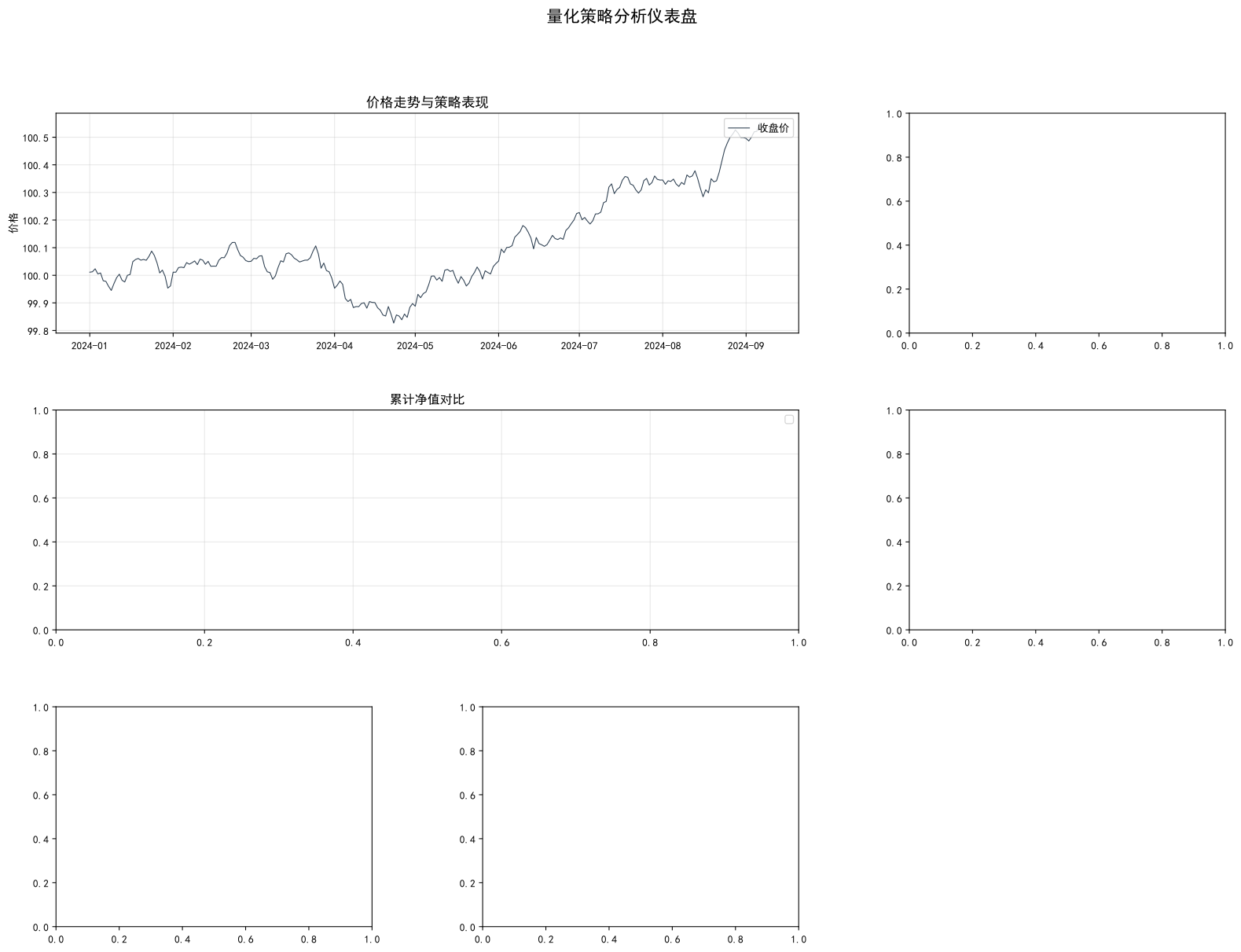
📘 本段代码定义了 1 个函数/类:函数 `quant_dashboard`(创建专业的量化策略仪表盘,整合多个关键诊断图表)。该片段为教学展示(未包含独立运行的输入数据),可在实战练习中结合真实数据调用。
案例3:因子分析可视化工具箱
此处有展示代码展开 ▼
python
import matplotlib.pyplot as plt
# 注:本案例纯 matplotlib + scipy, 不依赖 seaborn(浏览器沙箱不支持)。
import numpy as np
import pandas as pd
from scipy import stats

def factor_analysis_viz(factor_values, forward_returns, factor_name='Factor',
                         n_quantiles=5, periods=None):
    """
    因子分析可视化套件

    factor_values: Series, 每期的因子值
    forward_returns: Series, 对应的未来一期收益率
    """
    # 对齐数据
    data = pd.DataFrame({
        'factor': factor_values,
        'fwd_return': forward_returns
    }).dropna()

    fig, axes = plt.subplots(2, 3, figsize=(18, 10))

    # === 1. 散点图+回归线 ===
    axes[0, 0].scatter(data['factor'], data['fwd_return'],
                      alpha=0.3, s=10, c='steelblue', edgecolors='none')

    # 添加分组均值线
    data['quantile'] = pd.qcut(data['factor'], n_quantiles, labels=False, duplicates='drop')
    group_means = data.groupby('quantile')[['factor', 'fwd_return']].mean()
    axes[0, 0].plot(group_means['factor'], group_means['fwd_return'],
                   'ro-', linewidth=2, markersize=8, label='分组均值')

    # OLS回归线
    slope, intercept, r_value, p_value, _ = stats.linregress(data['factor'], data['fwd_return'])
    x_range = np.linspace(data['factor'].min(), data['factor'].max(), 100)
    axes[0, 0].plot(x_range, intercept + slope * x_range, 'r-', linewidth=1.5,
                   alpha=0.5, label=f'OLS (R={r_value:.3f}, p={p_value:.4f})')

    axes[0, 0].axhline(y=0, color='black', linewidth=0.5, linestyle='--')
    axes[0, 0].set_xlabel('因子值')
    axes[0, 0].set_ylabel('未来收益')
    axes[0, 0].set_title(f'{factor_name}: 因子-收益散点图')
    axes[0, 0].legend(fontsize=8)
    axes[0, 0].grid(True, alpha=0.3)

    # === 2. 分位数收益柱状图 ===
    quantile_returns = data.groupby('quantile')['fwd_return'].mean()
    quantile_std = data.groupby('quantile')['fwd_return'].std() / np.sqrt(data.groupby('quantile').size())

    colors_bar = ['#e74c3c' if x < 0 else '#2ecc71' for x in quantile_returns]
    axes[0, 1].bar(range(len(quantile_returns)), quantile_returns.values,
                  color=colors_bar, edgecolor='white', yerr=quantile_std.values,
                  capsize=5, alpha=0.8)
    axes[0, 1].axhline(y=0, color='black', linewidth=0.5)
    axes[0, 1].set_xticks(range(len(quantile_returns)))
    axes[0, 1].set_xticklabels([f'Q{i+1}\n(低)' if i==0 else f'Q{i+1}\n(高)' if i==len(quantile_returns)-1 else f'Q{i+1}'
                                for i in range(len(quantile_returns))])
    axes[0, 1].set_ylabel('平均未来收益')
    axes[0, 1].set_title(f'{factor_name}: 分位数收益 (Q1-Q{n_quantiles})')
    axes[0, 1].grid(True, alpha=0.3)

    # === 3. Q-Q图 (因子值分布) ===
    stats.probplot(data['factor'], dist='norm', plot=axes[0, 2])
    axes[0, 2].set_title(f'{factor_name}: Q-Q图 (正态性检验)')
    axes[0, 2].grid(True, alpha=0.3)

    # === 4. 因子IC序列 (滚动) ===
    # 计算滚动Rank IC
    if len(data) > 60:
        rolling_ic = data['factor'].rolling(60).corr(data['fwd_return'])  # 默认 Pearson;若需 Spearman 改用 rolling(60).apply(lambda x: x.corr(x, method='spearman'))
        axes[1, 0].plot(rolling_ic.index, rolling_ic.values, linewidth=0.8, color='#2980b9')
        axes[1, 0].axhline(y=0, color='black', linewidth=0.5)
        axes[1, 0].axhline(y=rolling_ic.mean(), color='red', linestyle='--', linewidth=1,
                          label=f'均值={rolling_ic.mean():.4f}')
        axes[1, 0].fill_between(rolling_ic.index, 0, rolling_ic.values,
                               where=rolling_ic.values > 0, color='green', alpha=0.2)
        axes[1, 0].fill_between(rolling_ic.index, 0, rolling_ic.values,
                               where=rolling_ic.values < 0, color='red', alpha=0.2)
        axes[1, 0].set_title(f'{factor_name}: 滚动60期Rank IC')
        axes[1, 0].set_ylabel('Rank IC')
        axes[1, 0].legend(fontsize=8)
        axes[1, 0].grid(True, alpha=0.3)

    # === 5. 累积分位数收益 ===
    # 计算每个分位数的累计收益
    cum_returns = {}
    for q in sorted(data['quantile'].unique()):
        mask = data['quantile'] == q
        cum_rets = (1 + data.loc[mask, 'fwd_return'].sort_index()).cumprod()
        cum_returns[q] = cum_rets

    # 使用热力图展示不同时期的分位数收益
    if 'date' in data.columns:
        pass  # 可以用seaborn heatmap展示时间序列

    for q, cum_ret in cum_returns.items():
        label = f'Q{q+1}'
        alpha_val = 1.0 if q in [0, len(cum_returns)-1] else 0.3
        linewidth = 2 if q in [0, len(cum_returns)-1] else 0.5
        axes[1, 1].plot(cum_ret.index, cum_ret.values, linewidth=linewidth,
                       alpha=alpha_val, label=label)

    axes[1, 1].set_title(f'{factor_name}: 各分位数累计收益')
    axes[1, 1].set_ylabel('累计收益')
    axes[1, 1].legend(fontsize=8)
    axes[1, 1].grid(True, alpha=0.3)

    # === 6. 因子分布 + 分组边界 ===
    axes[1, 2].hist(data['factor'], bins=50, density=True, color='steelblue',
                   alpha=0.6, edgecolor='white')

    # 标注分位数边界
    for q in range(1, n_quantiles):
        boundary = data['factor'].quantile(q / n_quantiles)
        axes[1, 2].axvline(x=boundary, color='red', linestyle='--',
                          linewidth=0.8, alpha=0.6)

    axes[1, 2].axvline(x=data['factor'].median(), color='red', linewidth=1.5,
                      label=f'中位数={data["factor"].median():.3f}')
    axes[1, 2].set_title(f'{factor_name}: 因子分布 (Q1-Q{n_quantiles}分位线)')
    axes[1, 2].legend(fontsize=8)
    axes[1, 2].grid(True, alpha=0.3)

    # 总标题
    fig.suptitle(f'因子分析: {factor_name}', fontsize=15, fontweight='bold', y=1.01)
    plt.tight_layout()
    plt.show()

    # 输出统计信息
    print("=" * 50)
    print(f"因子分析: {factor_name}")
    print("=" * 50)
    print(f"样本量: {len(data)}")
    print(f"Rank IC: {data['factor'].corr(data['fwd_return'], method='spearman'):.4f}")
    print(f"OLS斜率: {slope:.6f}, R={r_value:.4f}, p={p_value:.4f}")
    print(f"Q1-Q{n_quantiles} 超额收益: {quantile_returns.iloc[-1] - quantile_returns.iloc[0]:.6f}")

    # 单调性检验
    mono_violations = np.sum(np.diff(quantile_returns.values) <= 0)
    print(f"分位数收益单调性违规数: {mono_violations}/{n_quantiles-1} (越低越好)")

    return {
        'rank_ic': data['factor'].corr(data['fwd_return'], method='spearman'),
        'ols_r': r_value, 'ols_p': p_value,
        'quantile_returns': quantile_returns,
        'long_short_spread': quantile_returns.iloc[-1] - quantile_returns.iloc[0]
    }

# 一键运行(用 demo 数据: factors 每列分别作为单独因子做分析)
result_momentum = factor_analysis_viz(
    factor_values=factors['momentum'],
    forward_returns=df['returns'].shift(-1).dropna(),
    factor_name='动量因子'
)
print(f"\n✅ 多空价差: {result_momentum['long_short_spread']:.4%} (rank IC: {result_momentum['rank_ic']:.3f})")点击展开可浏览运行结果
==================================================
因子分析: 动量因子
==================================================
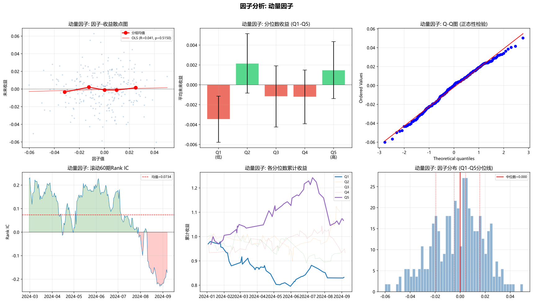
样本量: 251
Rank IC: 0.0497
OLS斜率: 0.040059, R=0.0413, p=0.5150
Q1-Q5 超额收益: 0.004943
分位数收益单调性违规数: 2/4 (越低越好)

✅ 多空价差: 0.4943%  (rank IC: 0.050)
常见误区
误区一:可视化只是"锦上添花"
事实:可视化往往是发现数据问题最有效的手段。一个Q-Q图可以在10秒内揭示偏离正态的程度,一个滚动IC图可以立即展示因子稳定性的变化。很多在做统计检验时被忽略的问题,在图上是一目了然的。
误区二:图表越花哨越好
事实:Tufte的"数据-墨水比"原则(Data-Ink Ratio)指出:图表中的墨水和像素应该主要用于展示数据,而非装饰。3D效果、过多的颜色渐变、不必要的动画——这些"图表垃圾 (chartjunk)"只会分散注意力。
误区三:默认设置就可以了
事实:matplotlib/seaborn的默认设置在金融场景下通常不合适:
- 默认颜色在打印时难以区分
- 没有对时间序列做特殊处理
- x轴标签在日期密集时会重叠
专业的金融图表需要定制:颜色方案、日期格式化、对数坐标轴、事件标注等等。
误区四:一张图能包含所有信息
事实:单一图表的信息量有限。好的量化可视化通常是多图联动的仪表盘,每张图表回答一个特定问题:回撤多大?收益分布如何?因子稳定性怎样?一张"综合图"试图回答所有问题,结果往往是哪个问题也没回答清楚。
实战练习
策略仪表盘:用你手上的一项策略回测数据,模仿quant_dashboard函数创建一个完整的分析仪表盘。确保包含:净值曲线、回撤曲线、收益分布直方图、月度收益热力图和关键统计指标。
因子可视化:取一个你感兴趣的量化因子(如20日反转、60日动量或换手率),使用factor_analysis_viz框架进行可视化分析。重点观察:(a) 因子值的分布是否正态,(b) 因子和未来收益的关系是否线性,(c) 分位数收益是否单调,(d) 滚动IC是否稳定。
交互式可视化:使用plotly库重新实现一个交互式的策略净值对比图,包含缩放、悬停提示和时间区间选择功能。比较静态图表和交互式图表在探索数据时的效率和体验差异。plotly需要
pip install plotly。
延伸阅读
- 《The Visual Display of Quantitative Information》—— Edward Tufte,信息可视化的圣经
- 《Storytelling with Data》—— Cole Nussbaumer Knaflic,数据叙事的实践指南
- matplotlib官方图库 (matplotlib.org/gallery) —— 大量可直接参考的代码示例
- 《Python Data Science Handbook》—— Jake VanderPlas,第4章matplotlib深入讲解
- Plotly官方文档 —— 交互式金融可视化的最佳选择
本章要点
- 可视化在量化中扮演探索、诊断和沟通三重角色,不是可有可无的装饰
- matploblib+seaborn是Python可视化的基础组合,plotly适合交互式分析
- 仪表盘式多图联动比单张大图更有洞察力,每张图回答一个特定问题
- 金融图表的颜色、标注、坐标轴需要专门定制,默认设置通常不够
- 可视化首先服务于分析者自己(发现问题),其次才服务于观众(表达结果)